Design, Model & Explore Approximate Arithmetic Circuits: A Tutorial

Multiobjective Optimization

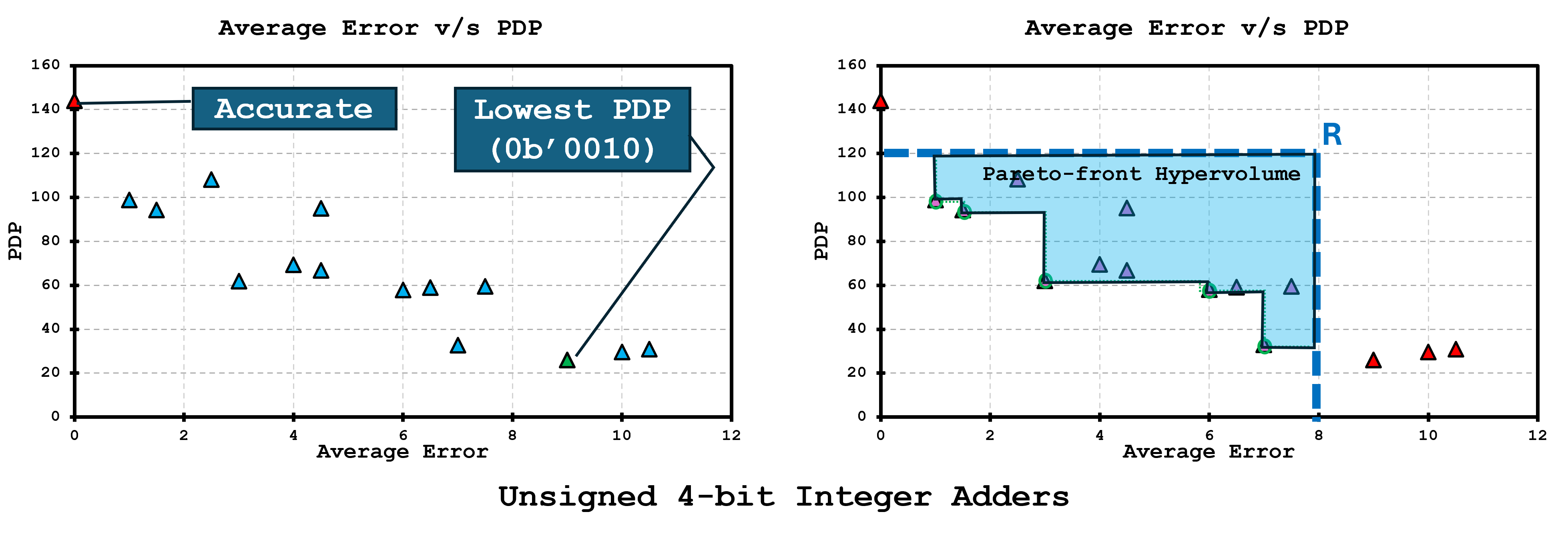
To make exploration concrete, we start with a toy but complete space: all realizations of an unsigned 4-bit adder produced by our pruning/variation knobs (Figure 1). The scatter on the left places every design in a two-objective plane (both axes minimized; e.g., an error metric vs. a cost metric such as power, delay, or PDP), marking the accurate baseline and a particularly efficient candidate. The right panel extracts the Pareto front (non-dominated designs) and shades the hypervolume with respect to a reference point R—a single number that grows as the frontier moves outward. We’ll use this example to illustrate how the tutorial evaluates search quality and convergence before scaling the same machinery to wider operators and application-level objectives.

Genetic Algorithm (GA) Search

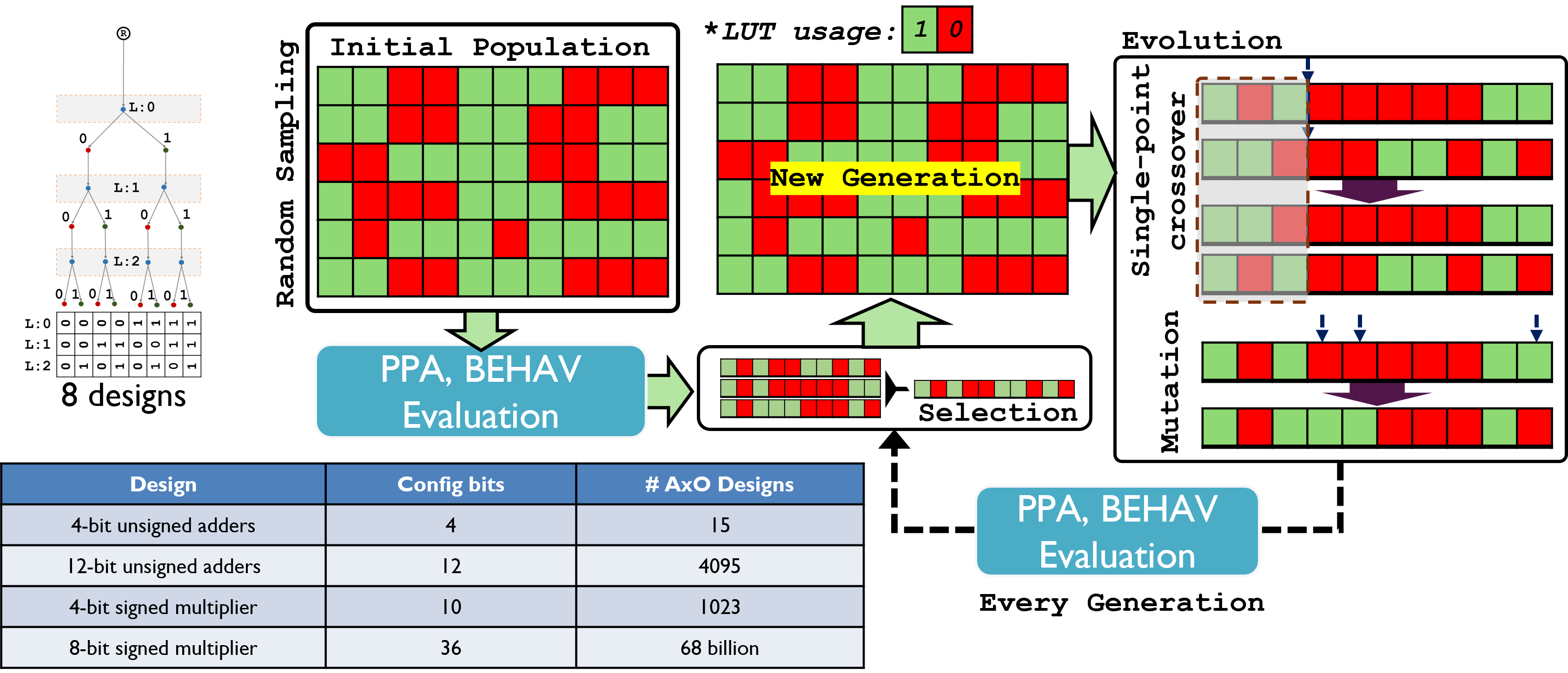
Once operators grow beyond toy widths, exhaustive enumeration explodes—from thousands to billions of AxO variants (bottom table). Figure 2 shows how we handle this with a genetic algorithm (GA): a population of bit-string designs is evaluated for PPA and BEHAV, then selected, crossed over (swapping contiguous slice ranges), and mutated (bit flips within legal neighborhoods) to form a new generation. Elites are preserved to keep the frontier from regressing, and legality checks/repairs ensure fabric-aware constraints (e.g., valid carry handoff) are never violated. This loop steadily pushes the Pareto front outward while sampling only a tiny fraction of the full space.

ML-based Surrogate

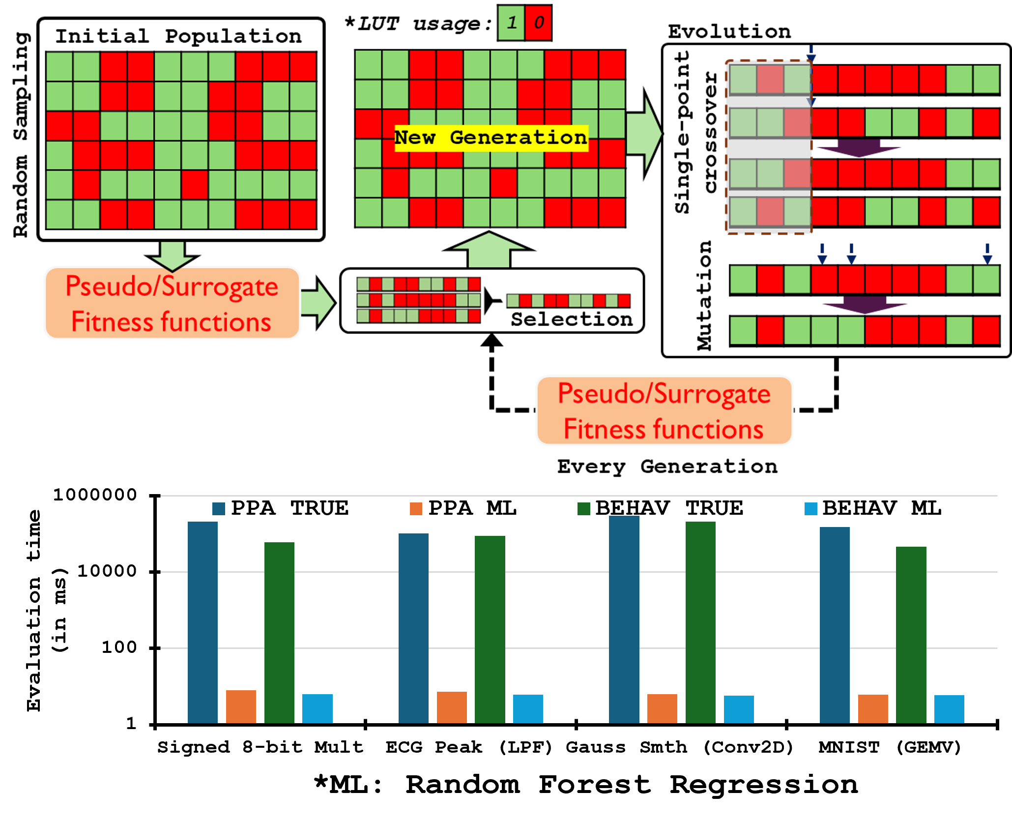
As design spaces explode, exact PPA/BEHAV evaluation for every individual becomes the bottleneck. Figure 3 shows how we insert ML-based surrogates (or “pseudo” fitness models) into the GA loop: populations of bit-string operators are decoded, but instead of synthesizing/simulating each one, we query learned regressors that predict power, delay, area, and error from the encoding (and a few structural features). This lets us rank and evolve candidates several orders of magnitude faster, reserving expensive ground-truth evaluations for selection, periodic calibration, and final verification.

The bar charts at the bottom emphasize the payoff: operator-level estimates are already faster than full synthesis/sim, but application-specific surrogates (that map operator sets → task accuracy/latency) produce even larger time savings—turning multi-hour pipelines into seconds per batch. With calibrated uncertainty, we can bias mutation/crossover toward regions where the model predicts large hypervolume gains yet remains uncertain, creating an active-learning loop that tightens the surrogate as the Pareto front advances.

GA using ML-Surrogate

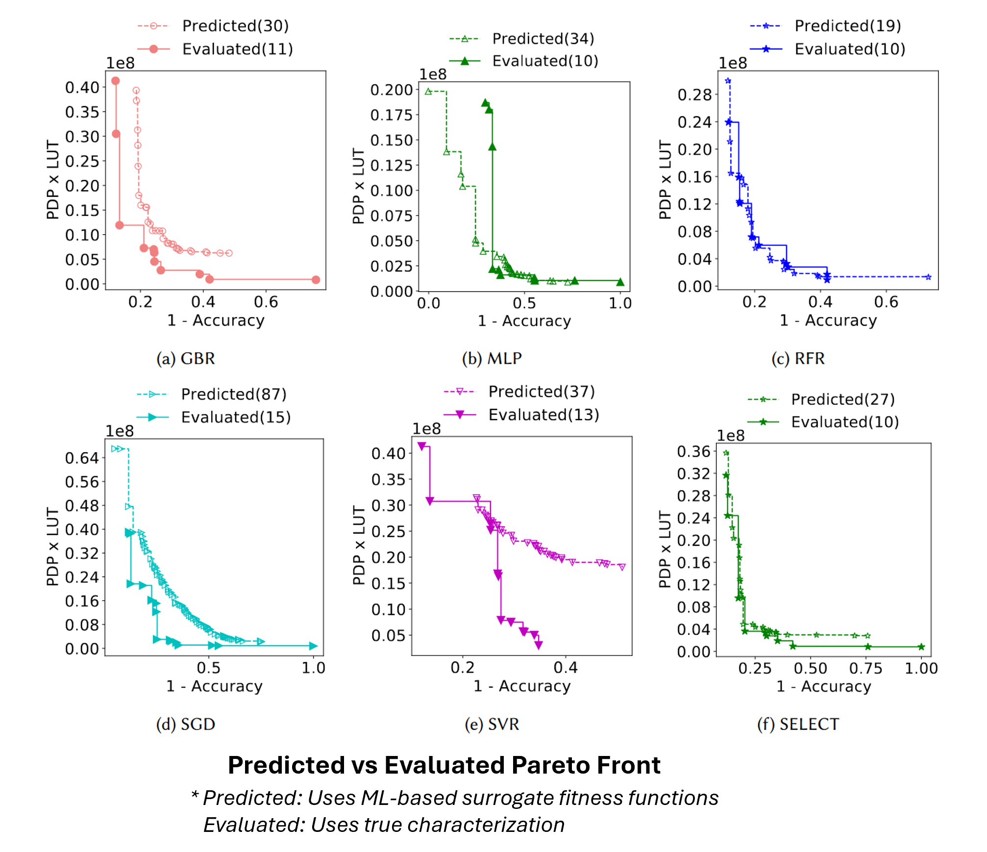
When we evolve with surrogate models, the GA advances a pseudo Pareto front—the set of candidates predicted to be non-dominated. Figure 4 compares that predicted front (dashed, “Predicted”) against the true front obtained after selective characterization (solid, “Evaluated”). Each panel tries a different learner—GBR, MLP, RFR, SGD, SVR—and the SELECT strategy (f) that picks the best-performing model per metric (e.g., one for error, another for power or PDP×LUT). In practice, we exploit the pseudo-front as a filter: only a budgeted subset of its points are synthesized/simulated per generation, correcting the surrogate and promoting the truly non-dominated designs. This closes the loop—fast search from predictions, reliability from targeted ground truth.

v1.0 @ ESWeek 2025, Taipei, Taiwan